Getting Started#

[35]:

from GaiaAlertsPy import alert as gaap

import numpy as np
from astropy.stats import sigma_clip
import matplotlib.pyplot as plt
%matplotlib inline
%config InlineBackend.figure_format = "retina"
from matplotlib import rcParams
rcParams['savefig.dpi'] = 550
rcParams['font.size'] = 20
plt.rc('font', family='serif')

# fancy plotting
import seaborn as sns
pal = sns.color_palette('magma', 80)
hex_colors = pal.as_hex()

Query all Gaia Photometric Science Alerts to Date#

[6]:

table = gaap.all_sources() # query and download all Gaia Photometric Science Alerts

[5]:

table

[5]:

Table length=25708

Name	Date	RaDeg	DecDeg	AlertMag	HistoricMag	HistoricStdDev	Class	Published	Comment	TNSid
str9	str19	float64	float64	float64	float64	float64	str14	str19	str130	str10
Gaia24byo	2024-07-21 08:45:07	189.20586	6.84128	18.44	--	--	unknown	2024-07-24 21:12:16	candidate SN near galaxy WISEA J123649.31+065027.9	AT2024poq
Gaia24byn	2024-07-21 00:34:35	32.8506	46.70412	18.3	--	--	unknown	2024-07-24 21:11:26	Apparently hostless transient	AT2024knb
Gaia24bym	2024-07-21 20:00:19	211.39828	-39.20317	18.48	--	--	SN	2024-07-24 21:10:36	confirmed SN in galaxy IC 4367	SN2024pfc
Gaia24byl	2024-07-21 13:37:09	233.02488	-60.3525	18.7	--	--	unknown	2024-07-24 21:09:46	blue transient in the galactic plane	AT2024qah
Gaia24byk	2024-07-21 15:21:38	172.17452	42.52083	18.86	19.34	0.11	QSO	2024-07-24 21:08:56	slow brightening in known QSO	AT2024qag
Gaia24byj	2024-07-21 05:07:36	23.56687	30.61165	17.47	17.97	0.15	unknown	2024-07-24 21:08:06	Brightening in Gaia and GALEX source	AT2020aafy
Gaia24byi	2024-07-21 19:29:51	248.02041	-64.88373	18.72	19.48	0.21	unknown	2024-07-24 21:07:04	Brightening of a Gaia and WISE source	AT2024qaf
Gaia24byh	2024-07-20 18:07:05	1.79692	-19.91794	18.94	19.28	0.09	unknown	2024-07-24 11:49:06	Brightening in Gaia and Wise source	AT2024pzq
Gaia24byg	2024-07-20 22:53:27	29.21525	42.50217	17.41	20.28	0.15	unknown	2024-07-24 11:43:54	2.5 mag brightening in candidate CV TCP J01565167+4230076	AT2024moh
Gaia24byf	2024-07-20 10:37:26	38.2396	55.66286	17.88	19.13	0.59	unknown	2024-07-24 11:41:44	1.5 mag brightening in candidate CV	AT2024pzp
...	...	...	...	...	...	...	...	...	...	...
Gaia14aaj	2014-09-12 15:40:38	187.7021	46.96982	18.98	19.56	0.1	unknown	2014-10-13 14:29:00	--	--
Gaia14aai	2014-08-30 11:57:30	23.88339	-20.40796	19.18	19.7	0.08	unknown	2014-10-13 14:29:00	--	--
Gaia14aah	2014-08-26 19:42:12	210.45337	54.5133	18.0	18.51	0.06	unknown	2014-10-13 14:29:00	--	--
Gaia14aag	2014-08-22 15:17:46	219.14335	44.65261	17.75	18.42	0.02	unknown	2014-10-13 14:29:00	--	--
Gaia14aaf	2014-08-17 21:35:53	244.25381	62.00685	17.05	18.06	0.19	CV	2014-10-13 14:29:00	--	--
Gaia14aae	2014-08-11 13:43:26	242.89156	63.14217	16.04	17.56	0.2	CV	2014-10-13 14:29:00	--	--
Gaia14aad	2014-08-08 01:17:01	209.68122	48.70098	18.28	18.85	0.02	unknown	2014-10-13 14:29:00	--	--
Gaia14aac	2014-08-02 07:19:24	214.66744	56.46959	18.68	19.55	0.05	unknown	2014-10-13 14:29:00	--	--
Gaia14aab	2014-07-27 19:10:29	206.91011	55.54871	19.11	20.0	0.1	unknown	2014-10-13 14:29:00	--	--
Gaia14aaa	2014-08-30 02:22:31	200.25961	45.53943	17.32	19.22	0.42	SN Ia	2014-09-12 09:00:00	--	--

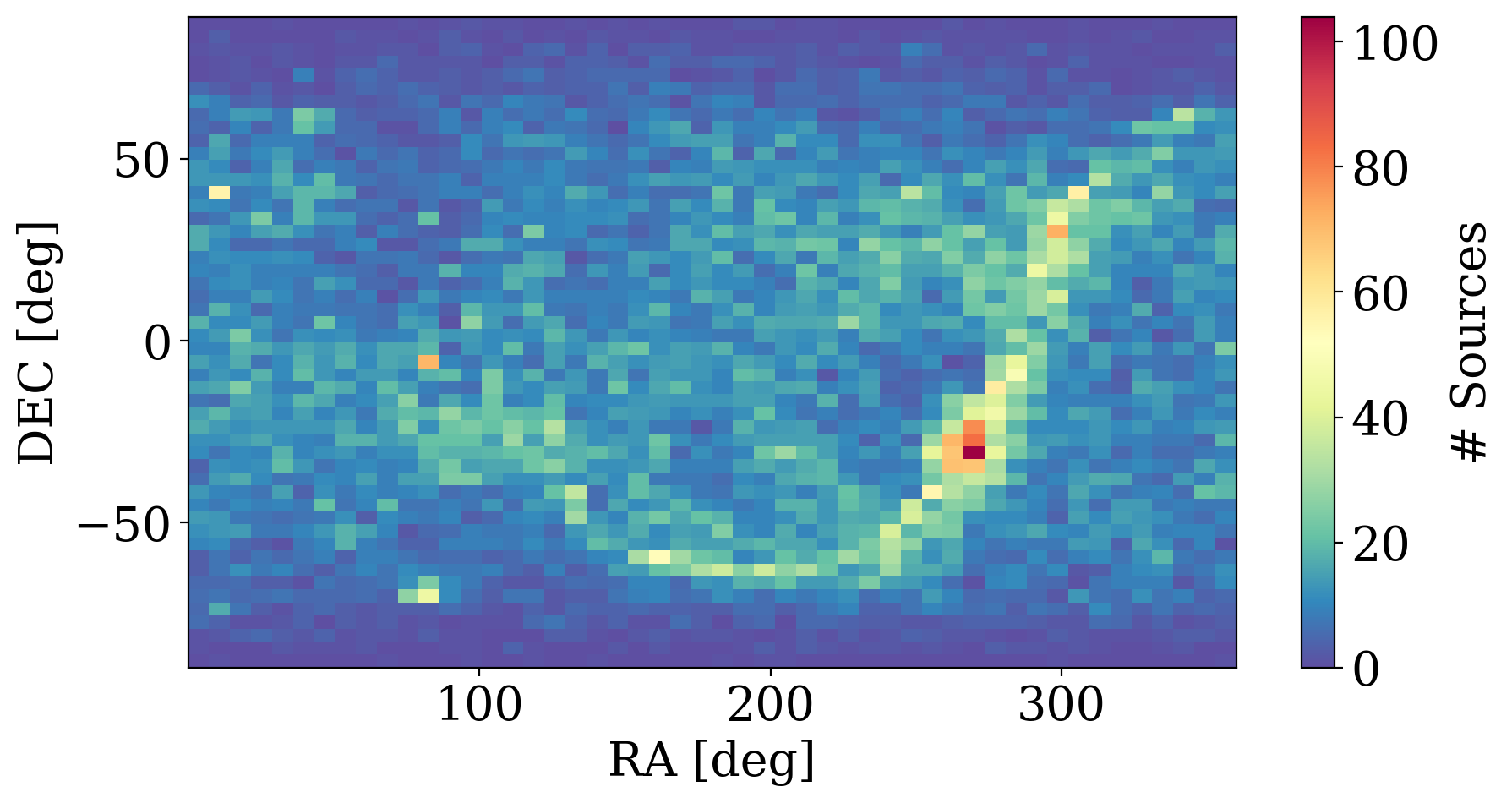
Sky Distribution of Alerts#

[6]:

plt.figure(figsize=(10,5))
_ = plt.hist2d(table['RaDeg'], table['DecDeg'], bins=(50, 50), cmap='Spectral_r')
plt.colorbar(label='# Sources')
plt.xlabel("RA [deg]")
plt.ylabel("DEC [deg]")

[6]:

Text(0, 0.5, 'DEC [deg]')

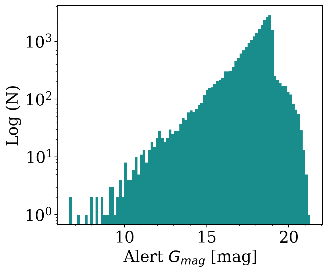
../_images/source_getting-started_6_1.png

Histogram of All Alert Magnitudes#

[11]:

plt.figure(figsize=(6,5))
_ = plt.hist(table['AlertMag'], histtype='stepfilled', color='teal', bins='scott', alpha=0.9)
plt.yscale('log')
plt.ylabel("Log (N)")
plt.xlabel("Alert $G_{mag}$ [mag]")
plt.minorticks_on()

../_images/source_getting-started_8_0.png

Getting Started with Alert Light Cuves#

In this short tutorial you will learn how to use GaiaAlertsPy and query the alert light curves. Once you query a Gaia Alerts, it will return a astropy.Table containing the epochal photometry.

[7]:

target_id = "Gaia22eoa"
alert_lc = gaap.GaiaAlert(target_id).query_lightcurve_alert()

[16]:

# view first 5 alerts
alert_lc[0:5]

[16]:

Table length=5

JD	mag_G	mag_G_error
float64	float64	float64
2457107.4551157407	16.7	0.015068630569774477
2457131.1310416665	16.89	0.01568925719710279
2457268.409351852	16.81	0.015420801849645116
2457298.7162152776	17.0	0.016077223994238388
2457319.6403819444	16.98	0.016004964926408682

The photometric uncertainties are calculated using the following equation and are valid for 13<G<21:

\[\begin{equation} \sigma_{mag_{G}} = 3.43779 - (G/1.13759) + (G/3.44123)^2 - (G/6.51996)^3 + (G/11.45922)^4 \end{equation}\]

For more information please see Gaia Early Data Release 3. Gaia photometric science alerts.

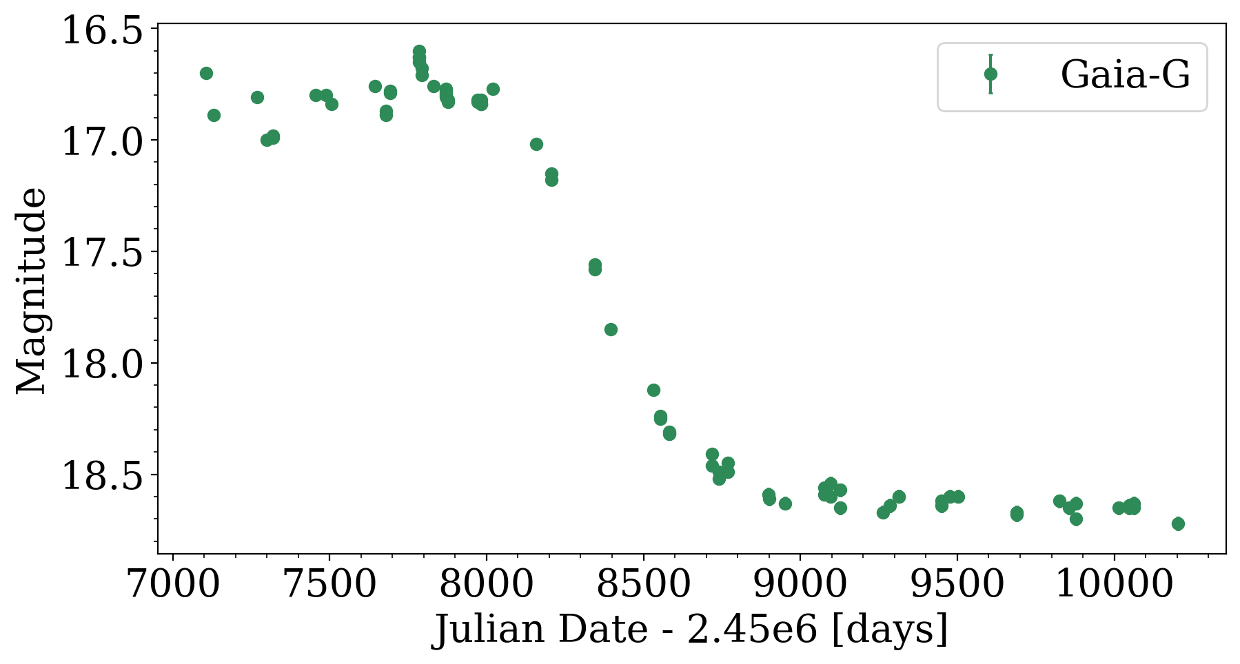
Let’s plot the light curve of this interesting Young Stellar Object:

[8]:

fig, ax = plt.subplots(nrows=1, ncols=1, figsize=(10,5))
ax.errorbar(alert_lc['JD']-2.45e6, alert_lc['mag_G'], alert_lc['mag_G_error'], fmt='o', capsize=1, color='seagreen',
label='Gaia-G')
ax.legend()
ax.set_ylim(ax.set_ylim()[::-1])
ax.set_xlabel("Julian Date - 2.45e6 [days]")
ax.set_ylabel("Magnitude")
plt.minorticks_on()

../_images/source_getting-started_14_0.png

Accessing the BP-RP Low-Res. Spectra#

For the moment we suggest that the spectra for each band is summed and the zero-point for each filter to be applied when converting from the raw ADU to the AB magnitude system. Further investigation will examine the calibration between standard stars and calibrating the ADU spectra to more reliable zero-point estimations and other systematics.

Warning – this is a very crude estimate to convert the BP/RP spectra to BP/RP magnitudes. More tutorials and methods for calibration will come soon!

Let’s first fetch all the BP/RP photometry:

[9]:

# Now we can even query the BP_RP information
color_lc = gaap.GaiaAlert(target_id).query_bprp_history()

[11]:

color_lc[0:5]

[11]:

Table length=5

Date	JD	Average Mag.	order	bp	rp	Name
str19	float64	float64	int64	float64[60]	float64[60]	str9
2015-03-25 22:55:22	2457107.46	16.7	0	0.0 .. 14.0	0.019 .. -2.419	Gaia22eoa
2015-04-18 15:08:42	2457131.13	16.89	1	1.2061 .. -0.2061	0.2057 .. -5.2057	Gaia22eoa
2015-09-02 21:49:29	2457268.41	16.81	2	1.9246 .. -2.3246	0.5859 .. -1.3859	Gaia22eoa
2015-10-03 05:11:22	2457298.72	17.0	3	2.9471 .. -0.5471	0.238 .. -3.038	Gaia22eoa
2015-10-24 03:22:10	2457319.64	16.98	4	-1.6875 .. 8.0875	-1.029 .. -4.771	Gaia22eoa

Now we can estimate a very approximate magnitude for each bp/rp spectrum using the instrumental zero-point values:

[29]:

# Instrumental zero-point values
zp_BP, zp_RP = 25.3514, 24.7619 # Table 5.2 (https://gea.esac.esa.int/archive/documentation/GDR2/Data_processing/chap_cu5pho/sec_cu5pho_calibr/ssec_cu5pho_calibr_extern.html)

bp_mag, rp_mag = [], []
for _lc in color_lc:
    bp0, rp0 = _lc['bp'], _lc['rp']

    # Count only positive ADU counts & apply 5-sigma clip (see Hodgkin et al. 2021; Section 3.6)
    bp, rp = sigma_clip(bp0[bp0>0], sigma=5), sigma_clip(rp0[rp0>0], sigma=5)

    # Convert total flux to magnitudes
    bp_mag.append(-2.5*np.log10(bp.sum()) + zp_BP)
    rp_mag.append(-2.5*np.log10(rp.sum()) + zp_RP)

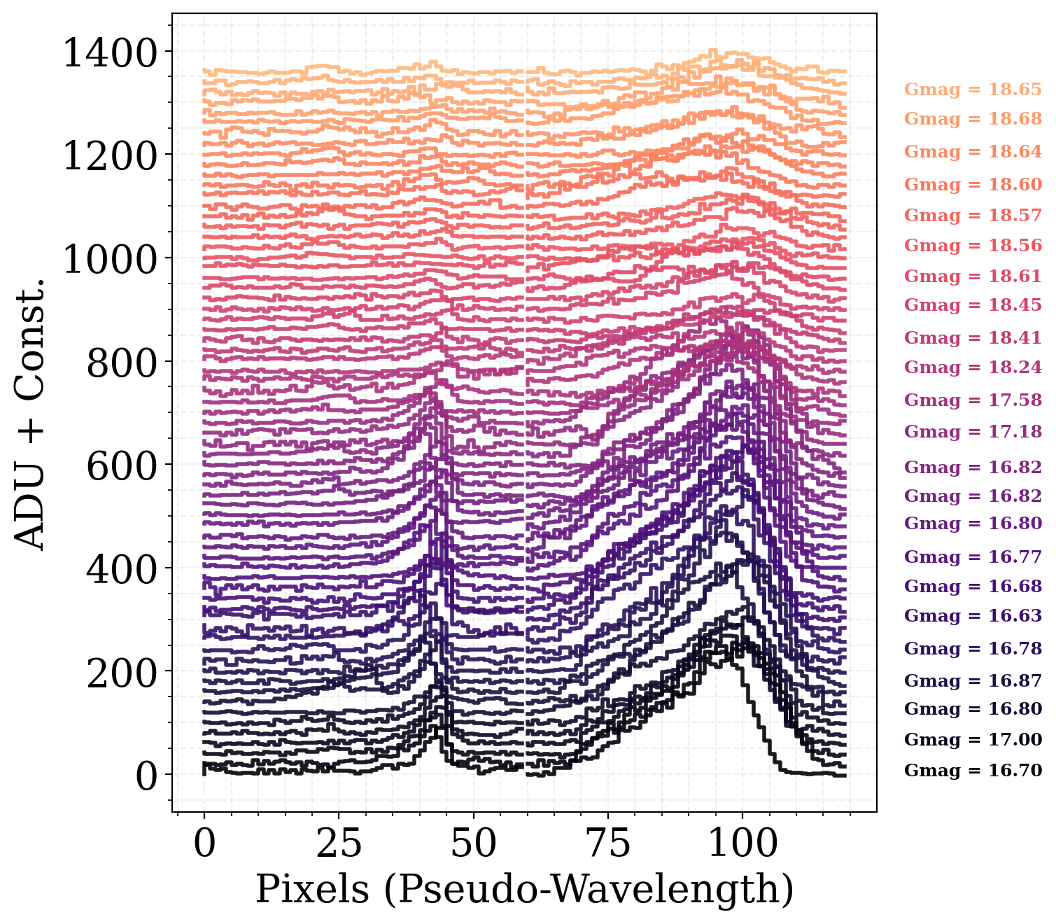
Time Series BP RP Spectra#

Alternatively, we can also fetch the raw ADU spectra that are reported on the GSA website. Same drill as before. These spectra are not calibrated - however some crude clolors can be extracted if you know the SED if your soruce.

Supposed we wanted to see the overall change in the low-res BP/RP spectra as a function of time and Gaia G magnitude. We can make a nice visualization combining the epochal BP/RP spectra including the average G band magnitude. From the plot below, we can see how for this particular souce that its spectrum is mostly red!

Please see the epochal BP/RP tutorial for more details!

[36]:

plt.figure(figsize=(8, 7))

# Plotting each color light curve
for i, c in enumerate(color_lc):
    offset = i * 20
    color = hex_colors[i % len(hex_colors)]

    # Plot BP and RP light curves with offset
    plt.step(range(0, 60), c['bp'] + offset, color=color, alpha=0.9, lw=2)
    plt.step(range(60, 120), c['rp'] + offset, color=color, alpha=0.9, lw=2)

    # Annotate with average magnitude every third curve
    if i % 3 == 0:
        plt.text(130, np.min(c['rp']) + offset, f"Gmag = {c['Average Mag.']:.2f}", fontsize=9, color=color, weight='bold')

# Labels and grid
plt.ylabel("ADU + Const.")
plt.xlabel("Pixels (Pseudo-Wavelength)")
plt.minorticks_on()
plt.grid(which='both', linestyle='--', alpha=0.2)

plt.tight_layout()

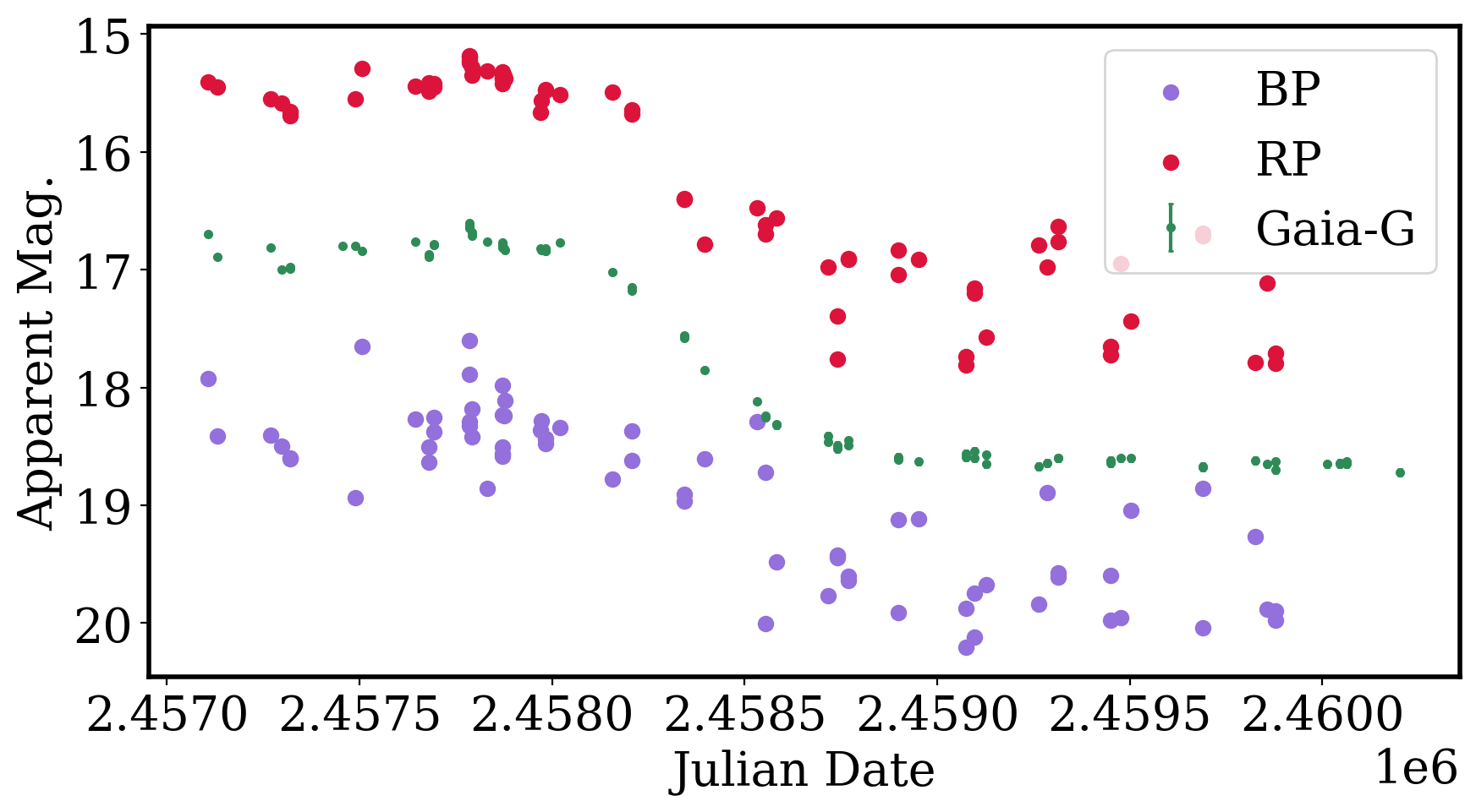
../_images/source_getting-started_22_0.png

Using the extrapolated BP/RP colors we can now plot the BP and RP light curves to see if our object of interest has any color evolution:

[33]:

fig, ax = plt.subplots(nrows=1, ncols=1, figsize=(10,5))
ax.errorbar(alert_lc['JD'], alert_lc['mag_G'], alert_lc['mag_G_error'], fmt='.', capsize=1, color='seagreen',
label='Gaia-G')
ax.scatter(color_lc['JD'], bp_mag, color='mediumpurple', label='BP')
ax.scatter(color_lc['JD'], rp_mag, color='crimson', label='RP')
ax.legend()
ax.set_ylim(ax.set_ylim()[::-1])
ax.set_xlabel("Julian Date")
ax.set_ylabel("Apparent Mag.")

[33]:

Text(0, 0.5, 'Apparent Mag.')

../_images/source_getting-started_24_1.png